Simulation Models
Fluorescence dynamics
The fluorescence dynamics in SASS are modeled as memoryless state systems. Such systems are comprised of two or more states that a fluorophore may occupy at any given time. During the course of an experiment, the fluorophore may randomly transition from its current state \(m\) to a new state \(n\), and the probability with which this transition occurs is determined partly by the so-called rate constant \(k_{mn}\).
Memorylessness means that the probability to transition to any accessible state does not depend on the time that the fluorophore has already spent in its current state. This assumption is well-founded: it is unlikely that a fluorescent molecule possesses some mechanism to keep track of time. Under the assumption of memorylessness, the length of the time interval \(t\) that is spent by a fluorophore in its current state \(S_m\) before making a transition to state \(S_n\) is given by an exponential probability density function
When multiple states are accessible from \(S_m\), then it may be shown that the probability that the fluorophore will have transitioned to the specific state \(S_n\) is
where \(K \equiv \sum_n k_{mn}\). Thus, the rate constants determine the relative probabilities of the transitions to different states.
Algorithm for state system simulations
The algorithm for simulating the state transitions proceeds as follows:
- The fluorescent molecule is assigned a pre-defined starting state \(S_m\).
- Next, a random transition time from the molecule’s current state is drawn for each accessible state \(n\) from an exponential distribution, \(\forall n : t_{mn} \sim \text{Exp} \left( \tau_{mn} \right)\) where \(\tau_{mn} \equiv 1 / k_{mn}\) is the average of the distribution.
- The smallest value from this set of transition times is computed and stored as the molecule’s transition time \(T \equiv \text{Min} \left( { t_{mn} }\right)\). The corresponding molecular state \(S_n\) is stored for use in the next step.
- The simulation time is advanced one time step. If, during this time, a total amount of time has elapsed that is greater than the previously calculated transition time \(T\), then the molecule is transitioned into its next state. The new next state and its transition time are generated and stored in the manner just described.
- This process is repeated as the simulation continues until a pre-determined number of time steps have occurred or it is stopped by the user.
Non-stationary state transitions
In PALM/STORM type experiments, one or more rate constants depend on the light irradiance (power per area) of one or more light sources. Indeed, adjusting the power during an acquisition is a common way to optimize the quality of datasets derived from such experiments because it offers a direct way to tune the density of fluorophores in a light-emitting state.
When the laser irradiance varies with time, so too do the rate constants and, therefore, the relative numbers of the fluorophores found in each state. Fortunately, the memorylessness property makes it easy to adapt the above algorithm to account for a changing irradiance. At each time step of the simulation, a check is performed to see whether the laser irradiance has changed. If it has, new rate constants are computed and a new transition time and state are derived from the algorithm described above.
State system representations
As an example of how state systems are represented in SASS, consider the simplified three-state fluorophore model pictured below.

In this simple model, the fluorophore may be in a fluorescence emitting (ON) state, a non-emitting (OFF) state, and an irreversibly bleached state from which it may never recover. (This model is perhaps too simplistic as it does not account for the typically numerous non-emitting states that real fluorophores possess. It does, however, capture the essential behavior in a SMLM experiment.)
The transition rate from OFF to ON is a constant, \(k_{ON}\), as is the rate \(k_{b}\) from the OFF to the BLEACHED state. The ON to OFF rate \(k_{OFF}\) is a function of the irradiance and may be expanded as
Let’s assume that \(k_{OFF}\) is at most linear with the irradiance. Then, the full dynamics of the fluorophore may be specified by a \(3 \times 3 \times 2\) matrix \(M\)
(Note that some browsers may not render the first elements of the above matrices. Both elements are 0.)
The rows of each matrix represent the state being transitioned from (ON, OFF, and BLEACHED states respectively), while the columns represent the state that is transitioned to (in the same order). For example, the first row of \(M_{:,:,1}\) indicates that \(k_{OFF,0}\) is the zero-order term for the rate coefficient polynomial expansion in \(I\) from the ON state to the OFF state. Here, row number one corresponds to the ON state and column number 2 corresponds to the OFF state. The corresponding element in the second matrix \(M_{:,:,2}\) is \(k_{OFF,1}\) and indicates that the rate coefficient is linearly proportional to the irradiance. If there were a third matrix \(M_{:,:,3}\) with a \(k_{OFF,2}\) element, then this would indicate a second-order polynomial term for the dependence of \(k\) on \(I\). Zeros for all the remaining elements in \(M_{:,:,2}\) indicate that no other rates depend on the irradiance.
Any fluorophore state system may be implemented in SASS by specifying the matrix \(M\).
Shot noise and sensor noise
There are two noise models employed by SASS: photon shot noise—which accounts for the quantum nature of fluorescence emission—and sensor noise. Sensor noise is based on the models described in these two documents:
- Basden, Haniff, and Mackay, “Photon counting strategies with low-light-level CCDs,” Mon. Not. R. Aston. Soc. 345, 1187-1197 (2003)
- The EMVA 1288 Standard
Sensor noise models in SASS currently do not account for spatial non-uniformities or defect pixels; each pixel is assumed independent from all other pixels. Furthermore, each pixel has identical statistical properties to all other pixels.
Additional assumptions employed in SASS include:
- The sensor is linear.
- Noise sources are wide sense stationary with respect to time and space.
- Only quantum efficiency is wavelength-dependent.
- Only dark current is temperature dependent.
Shot noise
Photon shot noise (or just shot noise) represents fluctuations in the number of photons incident on a pixel between different frame exposures. It is due to the quantum nature of fluorescence emission and is not dependent upon any properties of the image sensor.
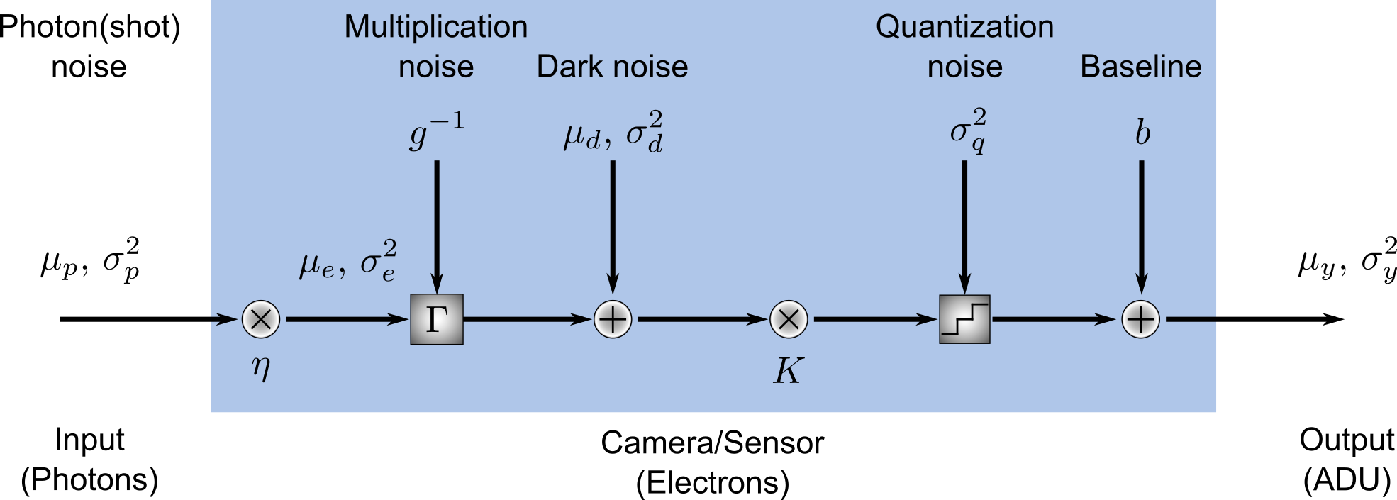
Let \(\mu_p\) represent the mean number of photons incident upon a pixel during the exposure of a given frame. The number of photoelectrons \(\mu_e\) generated by these photons is given by
where \(\eta\) is the quantum efficiency of the sensor and, in general, depends on the wavelength of the light.
Fluorescence emission is well-modeled as a Poisson process. Under this condition, the mean number of photoelectrons will be equivalent to the variance \(sigma_e^2\) of the number of photoelectrons generated over time.
Sensor temporal noise
Within the sensor, photoelectrons are converted to analog-to-digital units (ADU) through a step-wise process involving
- the amplification of the signal and the addition of multiplication noise (for cameras possessing a multiplication register),
- the addition of dark noise, which consists of readout noise and dark current noise,
- the conversion of electrons to voltages by multiplication with a constant system gain factor,
- and quantization of the voltage to discrete ADU values and summation with a constant baseline value.
The number of photoelectrons that is generated within the pixels of an electron multiplying CCD (EMCCD) is amplified within a serial register via electron avalanche multiplication. This process is random and introduces a multiplicative noise that is modeled as a gamma distribution \(\Gamma \left( \mu_e, g^{-1} \right)\) where \(g^{-1}\) is the inverse value of the camera’s EM gain. (Note that in some notations the second parameter of the gamma distribution is denoted directly by the gain, not its inverse.) Sensors such as sCMOS cameras that lack a serial multiplication register are modeled in SASS by setting the EM gain value to 0.
Following the multiplication register, dark current noise is added to the signal to account for thermally excited electrons within the pixels. Dark current is modeled as a zero-mean Gaussian distribution whose standard deviation is a free parameter. Typically, the value for this parameter is found by assuming that dark current is also a Poisson process whose variance is equivalent to the mean number of dark current electrons \(\mu_I t_{exp}\). Here, \(\mu_I\) is the dark current in electrons per time and \(t_{exp}\) is the exposure time of the frame. \(\mu_I\) is dependent on temperature in general. Dark current is often negligible in microscopy experiments, so it may often be safely ignored.
The total number of amplified photoelectrons and dark current electrons are then readout as a voltage, which introduces a readout noise. Readout noise is modeled as a zero-mean Gaussian distribution whose standard deviation is also a free parameter. The value for this parameter is often given on camera specification sheets as a median or root-mean-square (RMS) number of electrons. (RMS readout noise is preferred for sCMOS cameras because of pixel-to-pixel variation in the values.) Some camera manufacturers will combine dark current and readout noise into a single noise source known as dark noise with mean \(\mu_d\) and variance \(\sigma_d^2\).
After addition of the readout noise, the voltage signal is amplified by another free parameter found on camera specification sheets, the system gain \(K\). Finally, the signal is quantized into discrete ADUs and optionally summed with a constant baseline \(b\) to prevent negative pixel values. This baseline is often about 100 ADU. The quantization noise is a uniform distribution with variance \(\sigma_q^2 = \frac{1}{12} \, ADU^2\). It is automatically accounted for in the code by converting from double to integer data types.